BVH for Collision Detection: From AABB to Optimal Hierarchies

Why Broad-Phase Exists (and why naive O(N²) dies at 10k objects)
Bounding Volume Hierarchy: The Data Structure That Scales
Topology Choices: Binary vs. Multi-Branch, Pointer vs. Array Layout
Construction Algorithms: From Naive to SAH-Optimal
Traversal Strategies for Collision Queries
The Static/Dynamic Dichotomy: Why One Tree Cannot Serve Two Masters
The Dual-BVH Architecture Preview

1. Why Broad-Phase Exists

The Pairwise Problem

Every collision detection system faces the same fundamental challenge: given N objects, determine which pairs might be colliding so the expensive narrow-phase (SAT, GJK, EPA) only runs on plausible candidates.

The naive approach tests every pair:

// Naive O(N²) broad-phase — dies at ~10k objects
std::vector<CollisionPair> broadPhaseNaive(const std::vector<Object*>& objects) {
    std::vector<CollisionPair> pairs;
    for (size_t i = 0; i < objects.size(); ++i) {
        for (size_t j = i + 1; j < objects.size(); ++j) {
            if (aabbOverlap(objects[i]->aabb, objects[j]->aabb)) {
                pairs.emplace_back(objects[i], objects[j]);
            }
        }
    }
    return pairs;
}

Complexity: $O(N²)$ AABB tests. At 60 Hz you have 16.67 ms/frame. At 120 Hz: 8.33 ms.

Objects (N)	Pairwise Tests	@ 3 ns/test	Frame Budget (60 Hz)
100	4,950	0.015 ms	Trivial
1,000	499,500	1.5 ms	Comfortable
10,000	49,995,000	150 ms	10x over budget
100,000	~5x10^9	15,000 ms	Impossible

Cache Miss Catastrophe

The pairwise loop doesn’t just do too much work, it does it poorly. Each iteration accesses two random objects in memory. With 10k objects, you’re thrashing L3 cache every frame. The BVH approach exploits spatial coherence: nearby objects in space are nearby in the tree, turning random access into sequential scans.

The Real Job: Proving Separation

KEY INSIGHT: Broad-phase is a rejection machine. Broad-phase is not about finding collisions. It’s about proving separation as cheaply as possible. Every AABB overlap test that returns false is a victory, you’ve eliminated a narrow-phase call for zero cost. The BVH’s job is to maximize these cheap rejections.

2. Bounding Volume Hierarchy: The Data Structure That Scales

Formal Definition

A Bounding Volume Hierarchy (BVH) is a tree where:

Leaf nodes store an object’s AABB (and object ID)
Internal nodes store the union AABB of their children
Invariant: Parent AABB fully contains all descendant AABBs (no gaps)

BVH Tree Structure

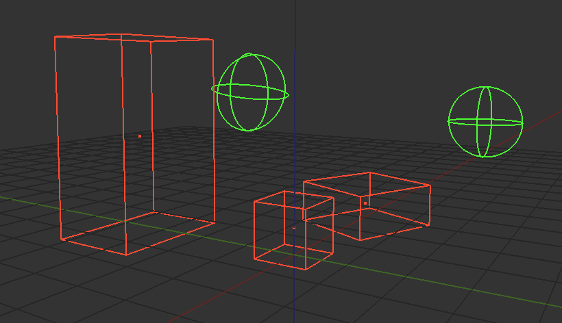physics collider

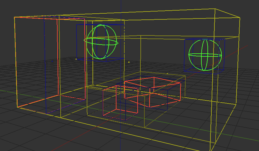BVH tree

Invariant: the parent AABB contains all descendants. A query traverses two trees simultaneously and early-outs the moment an AABB-overlap test on a node pair fails.

Collision Detection Query: The Key Difference from Ray Tracing

Ray tracing traverses one BVH with a ray, stopping at the closest hit. Collision detection traverses two BVHs simultaneously (or one BVH vs. query volume), collecting all overlapping pairs. No early termination on “closest” we need the complete set.

void traverseBVHvsBVH(const BVHNode* a, const BVHNode* b, 
                      std::vector<CollisionPair>& out) {
    if (!aabbOverlap(a->bounds, b->bounds)) return;  // Proved separation
    
    if (a->isLeaf && b->isLeaf) {
        out.emplace_back(a->objectId, b->objectId);
        return;
    }
    
    // Recurse into children 
    if (a->isLeaf || (!b->isLeaf && b->depth > a->depth)) {
        traverseBVHvsBVH(a, b->left, out);
        traverseBVHvsBVH(a, b->right, out);
    } else {
        traverseBVHvsBVH(a->left, b, out);
        traverseBVHvsBVH(a->right, b, out);
    }
}

Memory Layout: Cache-Friendly First

Layout	Pros	Cons	Best For
Pointer-based (`Node* left, right`)	Flexible, easy dynamic modification	Cache misses, allocation overhead	Prototyping
Array-based / SoA (separate arrays for min/max/children)	Maximum SIMD, perfect prefetch	Fixed topology, complex refit	Static trees, GPU
Hybrid: Array of structs with indices	Cache-friendly, supports rebuild, SIMD-ready	Slightly larger nodes	Production CPU

3. Topology Choices: Binary vs. Multi-Branch

Branching Factor Trade-offs

Factor	BVH2 (Binary)	BVH4	BVH8
Tree depth	log₂(N)	log₄(N)	log₈(N)
SIMD width	2-wide (SSE)	4-wide (AVX2)	8-wide (AVX-512)
Internal node size	32 bytes	64 bytes	128 bytes
False positive rate	Lowest	Medium	Highest
Leaf pairs tested	Fewest	More	Most
Construction complexity	Simple	Moderate	Complex

Collision-Specific Insight

For ray tracing: traversal depth dominates (early termination on closest hit). Wider = better.

For collision detection: leaf pair count dominates (no early termination, need all overlaps). Wider BVH = larger internal AABBs = more false positives = more narrow-phase calls.

Expected node visits ≈ (branching_factor)^depth × false_positive_rate
                     ≈ N^(1/log₂(branching_factor)) × (1 + ε×branching_factor)

Recommendation: BVH2 or BVH4 for CPU collision. BVH8+ only for GPU ray tracing where traversal depth matters more than pair count.

4. Construction Algorithms: From Naive to SAH-Optimal

Building a Bounding Volume Hierarchy (BVH) is a balancing act between build speed and tree quality. A high-quality tree renders frames much faster, but takes longer to construct.

4.1 Naive Top-Down (Median Split)

The simplest way to build a BVH is to divide and conquer using the median split method:

Find the longest axis of the current bounding box (X, Y, or Z).
Sort all objects along this axis based on their center points.
Split the list exactly in half, putting 50% of the objects in the left child and 50% in the right child.
Recurse until you hit a leaf node.

Complexity: $O(N log N)$ .

Flaw: Splits by object count, not surface area. Clusters produce terrible trees.

BVHNode* buildMedian(std::vector<Object*>& objects, int start, int end) {
    if (end - start == 1) return createLeaf(objects[start]);
    
    // Find longest axis
    AABB bounds = computeBounds(objects, start, end);
    int axis = longestAxis(bounds);
    
    // Sort by centroid on that axis
    std::sort(objects.begin() + start, objects.begin() + end,
        [axis](Object* a, Object* b) {
            return a->aabb.centroid()[axis] < b->aabb.centroid()[axis];
        });
    
    int mid = start + (end - start) / 2;
    BVHNode* left  = buildMedian(objects, start, mid);
    BVHNode* right = buildMedian(objects, mid, end);
    return createInternal(left, right);
}

4.2 Surface Area Heuristic (SAH) - The Gold Standard

Instead of just checking the median, the SAH algorithm sweeps across the axis, evaluating the cost equation at different intervals or at every single object boundary. It then picks the exact split plane that yields the lowest mathematical cost.

Cost model: Expected cost of traversing a node:

$C = C_{trav} + \frac{SA(L)}{SA(P)} N_L C_{isct} + \frac{SA(R)}{SA(P)} N_R C_{isct}$

Where:

$C_{trav}$ : Cost of traversing a node.
$C_{isct}$ : Cost of intersecting a primitive.
$SA(P), SA(L), SA(R)$ : Surface area of the Parent, Left child, and Right child.
$N_L, N_R$ : Number of primitives in the left and right children.

Complexity: $O(N log² N)$ with spatial sorting, $O(N² log N)$ naive. Optimal quality.

Verdict: Slow to build, but produces structurally optimal trees. It is the gold standard for static scene geometry.

Full SAH Build Algorith

BVHNode* buildSAH(std::vector<Object*>& objects, int start, int end) {
    if (end - start == 1) return createLeaf(objects[start]);
    
    AABB totalBounds = computeBounds(objects, start, end);
    int bestAxis = -1;
    int bestSplit = -1;
    float bestCost = INFINITY;
    
    // Try all 3 axes
    for (int axis = 0; axis < 3; ++axis) {
        // Sort by centroid on this axis
        std::sort(objects.begin() + start, objects.begin() + end,
            [axis](Object* a, Object* b) {
                return a->aabb.centroid()[axis] < b->aabb.centroid()[axis];
            });
        
        // Evaluate EVERY split position (not just bins)
        AABB leftBounds, rightBounds = totalBounds;
        for (int i = start + 1; i < end; ++i) {
            leftBounds.expand(objects[i-1]->aabb);
            rightBounds = computeBounds(objects, i, end);
            
            float pLeft  = leftBounds.surfaceArea()  / totalBounds.surfaceArea();
            float pRight = rightBounds.surfaceArea() / totalBounds.surfaceArea();
            float cost = C_TRAV + pLeft * (i - start) * C_ISCT + pRight * (end - i) * C_ISCT;
            
            if (cost < bestCost) {
                bestCost = cost; bestAxis = axis; bestSplit = i;
            }
        }
    }
    
    // Partition at best split, recurse
    std::nth_element(objects.begin() + start, objects.begin() + bestSplit, objects.begin() + end,
        [bestAxis](Object* a, Object* b) {
            return a->aabb.centroid()[bestAxis] < b->aabb.centroid()[bestAxis];
        });
    
    return createInternal(
        buildSAH(objects, start, bestSplit),
        buildSAH(objects, bestSplit, end)
    );
}

4.3 Linear BVH (LBVH) / Morton Codes

LBVH builds the tree from the bottom up in linear time using a clever spatial hashing trick: Morton Codes. By taking the binary bits of an object’s 3D coordinates (X, Y, Z) and interleaving them, we map 3D space into a 1D integer.

Complexity: $O(N)$

Trade-off: 30-50% worse SAH cost vs. full SAH, but 10-100× faster build. Good for dynamic rebuilds; poor for static tree quality.

Watch this for a detailed explanation.

4.4 HLBVH (Hierarchical LBVH)

HLBVH offers the best of both worlds. It uses the ultra-fast LBVH Morton code method to group small clusters of objects at the bottom of the tree, and then uses the high-quality SAH method to build the top levels of the tree. This results in near-optimal speeds with incredibly fast build times.

LBVH for large clusters + SAH for small clusters. Best of both: near-SAH quality, near-LBVH speed.

4.5 Parallel Construction

Task graph: partition objects → build subtree per task → merge. Ideal: $O(N log N / P)$ , synchronization overhead real.

Algorithm	Build Time	Tree Quality (SAH)	Parallelizability
Median Split	Fast	Poor	Easy
Full SAH (optimal)	Slow	Optimal	Moderate
LBVH	Very Fast	30-50% worse	Trivial (radix sort)
HLBVH	Fast	Near-optimal	Good
Parallel SAH	Fast (scales)	Optimal	Good (TBB/job system)

5. Traversal Strategies for Collision Queries

The three traversal families below solve different query shapes. Their trade-offs are summarized first, then detailed in code.

Strategy	Use Case	Memory	Collision?
Iterative Pair (BVH vs BVH)	Two-world / self-collision	Stack	Yes (all pairs)
Stackless (BVH vs AABB)	Raycast, frustum, sweep	Zero stack	Single tree
SIMD BVH4 (BVH vs AABB)	High-throughput queries	SoA layout	Single tree
Front-to-Back	Ray tracing	Priority queue	No (wrong model)
Depth-First	Collision	Stack	Yes (all pairs)

5.1 BVH vs. BVH (Two-World / Self-Collision)

Simultaneous traversal of two trees. Stack of node pairs. Early-out on AABB overlap test.

void traverseBVHvsBVHIterative(const BVH& a, const BVH& b, 
                                std::vector<CollisionPair>& out) {
    struct StackEntry { uint32_t nodeA, nodeB; };
    std::vector<StackEntry> stack;
    stack.reserve(256);
    stack.push_back({0, 0});  // Root indices
    
    while (!stack.empty()) {
        auto [ia, ib] = stack.back(); stack.pop_back();
        const BVHNode& na = a.nodes[ia];
        const BVHNode& nb = b.nodes[ib];
        
        if (!aabbOverlap(na.bounds, nb.bounds)) continue;
        
        if (na.isLeaf && nb.isLeaf) {
            out.emplace_back(na.objectId, nb.objectId);
        } else if (na.isLeaf) {
            stack.push_back({ia, nb.left});
            stack.push_back({ia, nb.right});
        } else if (nb.isLeaf) {
            stack.push_back({na.left, ib});
            stack.push_back({na.right, ib});
        } else {
            // Both internal 
            // push all 4 combinations
            stack.push_back({na.left,  nb.left});
            stack.push_back({na.left,  nb.right});
            stack.push_back({na.right, nb.left});
            stack.push_back({na.right, nb.right});
        }
    }
}

5.2 BVH vs. Query Volume (Raycast / Sweep / Frustum)

Single-tree traversal with query volume. Key difference from ray tracing: no “closest hit” termination we need all overlaps.

5.3 Stackless Traversal (Pointerless / Index-Based)

Parent index stored in node → no explicit stack needed.

void traverseStackless(const BVH& bvh, const AABB& query, 
                       std::vector<uint32_t>& out) {
    uint32_t node = 0;  // Start at root
    uint32_t prev = UINT32_MAX;
    
    while (node != UINT32_MAX) {
        const BVHNode& n = bvh.nodes[node];
        
        // Coming down from parent
        if (prev == (node == 0 ? UINT32_MAX : bvh.nodes[node].parent)) {
            if (!aabbOverlap(n.bounds, query)) {
                // go to sibling or up
                node = (n.isLeaf || n.right == UINT32_MAX) ? n.parent : n.right;
            } else if (n.isLeaf) {
                out.push_back(n.objectId);
                node = (n.right == UINT32_MAX) ? n.parent : n.right;
            } else {
                node = n.left;  
            }
        }
        // Coming up from left child
        else if (prev == n.left) {
            node = (n.right == UINT32_MAX) ? n.parent : n.right;
        }
        // Coming up from right child
        else {
            node = n.parent;
        }
        prev = (node == UINT32_MAX) ? UINT32_MAX : node;
    }
}

Trade-off: More instructions per node, but zero stack allocation, cache-friendly.

5.4 Front-to-Back vs. Depth-First Ordering

Ordering	Ray Tracing	Collision Detection
Front-to-back	Enables early termination	No benefit (need all pairs)
Depth-first	Misses early termination	Cache-friendly, simple
Breadth-first	High memory	High memory

Insight: Collision BVH traversal is simpler than ray tracing (no closest-hit logic) but does more work (must visit all overlapping nodes).

6. The Static/Dynamic Dichotomy

---
config:
  theme: base
  flowchart:
    nodeSpacing: 26
    rankSpacing: 40
    curve: linear
    htmlLabels: false
    useMaxWidth: false
  themeVariables:
    background: '#0a0a0a'
    primaryColor: '#101010'
    primaryTextColor: '#e8e8e8'
    primaryBorderColor: '#3a3a3a'
    lineColor: '#4a4a4a'
    secondaryColor: '#101010'
    tertiaryColor: '#101010'
    mainBkg: '#101010'
    secondBkg: '#0d0d0d'
    tertiaryBkg: '#101010'
    nodeBorder: '#3a3a3a'
    clusterBkg: '#0d0d0d'
    clusterBorder: '#2a2a2a'
    titleColor: '#e8e8e8'
    edgeLabelBackground: '#0a0a0a'
    fontFamily: 'ui-monospace, SFMono-Regular, Menlo, Consolas, monospace'
    fontSize: '12px'
---
flowchart TD
    
    subgraph STATIC["STATIC GEOMETRY"]
        SC["Immutable scene<br/>100k–10M objects<br/>SAH built once<br/>then O(1) per query"]
    end
    subgraph DYNAMIC["DYNAMIC OBJECTS"]
        DC["Moves every frame<br/>100–10k objects<br/>tree quality decays"]
    end
    subgraph FAIL["SINGLE-TREE FAILURE"]
        F["Mixed scenes:<br/>rebuild cost explodes<br/>no single strategy fits both"]
    end
    subgraph SOL["DUAL-BVH SOLUTION"]
        DS["Static pipeline<br/>0 ms per frame"]
        DD["Dynamic pipeline<br/>insert + treelet refit"]
        JT["Joint traversal<br/>S-S · S-D · D-D pairs"]
        NP["Narrow phase<br/>SAT · GJK · EPA"]
    end

    SC --> DS
    DC --> DD
    DS --> JT
    DD --> JT
    JT --> NP
    F -.-|"avoids"| SOL

    classDef st fill:#101010,stroke:#808080,stroke-width:1px,color:#e8e8e8,padding:16px
    classDef dy fill:#101010,stroke:#b48ead,stroke-width:1px,color:#e8e8e8,padding:16px
    classDef fl fill:#0a0a0a,stroke:#4a4a4a,stroke-width:1px,stroke-dasharray:4 4,color:#808080,padding:16px
    classDef sl fill:#101010,stroke:#3a3a3a,stroke-width:1px,color:#e8e8e8,padding:16px
    classDef key fill:#141414,stroke:#e8e8e8,stroke-width:1.5px,color:#e8e8e8,padding:16px
    class SC st
    class DC dy
    class F fl
    class DS,DD,NP sl
    class JT key

6.1 Static Geometry Characteristics

World mesh, level geometry, baked props
Immutable at runtime
Massive count: 100k-10M triangles/objects
Quality requirement: Optimal SAH (built once, queried millions of times)
Build cost amortization: O(N log N) once → O(1) per frame forever

6.2 Dynamic Objects Characteristics

Characters, vehicles, debris, projectiles
Transform every frame (translation + rotation)
Moderate count: 100-10k objects
Quality degradation: Insertion inflates AABBs → tree quality decays
Rebuild frequency: Every frame (costly) vs. incremental (degrading)

6.3 The Single-Tree Failure Modes

Scenario	Single Tree Result
Static-heavy (1M static, 1k dynamic)	Rebuilding 1M nodes/frame = impossible
Dynamic-heavy (10k dynamic, 1k static)	Static objects pollute dynamic tree quality
Mixed	No optimal strategy exists

6.4 Quantitative Case Study

100k static triangles + 5k dynamic objects
Single tree rebuild: ~50 ms/frame (unacceptable)
Dual tree: Static 0 ms/frame, Dynamic 0.5 ms/frame (with incremental updates)

7. The Dual-BVH Architecture Preview

The Problem Statement

We need:

Static tree: Optimal SAH build, zero runtime cost, queried millions of times
Dynamic tree: Incremental updates, bounded quality degradation
Safe concurrent reconstruction: Readers never block, writers never wait

Three Innovations Previewed

Dual-BVH separation: Static and dynamic pipelines completely independent
Amortized treelet reconstruction : O(1) frame cost via bounded k treelets rebuilt per frame
**epoch system **: Read and write separation.

What Part 2 Will Cover

Full system mechanics: static tree construction pipeline, dynamic tree greedy insertion with degradation tracking, treelet rebuild ,Intrusive linked lists, epoch system, frame pipeline integration.

Resources & Further Learning

Video Tutorials

Building Collision Simulations - Reducible
Watch on YouTube →
Coding Adventure: Optimizing a Ray Tracer by Building a BVH - Sebastian Lague
Watch on YouTube →

Articles & Documentation

Bounding Volume Hierarchies - University of Illinois
Read the article →
Real-Time Collision Detection - Christer Ericson
Read Chapter 6 →

Table of Contents